A guide to practical data mining, collective intelligence, and building recommendation systems by Ron Zacharski.
Chapter 1 Introduction
Introduction to data mining. What it is. How it is used. What you will be able to do once you read this book.
Data mining is focused on finding patterns in data.
This book—the one you are holding—is intended more as a quick, gritty, hands-on introduction designed to give you a basic foundation of data mining techniques. Later, you can pick up a more comprehensive book to fill in any gaps that you wish.
Chapter 2: Get Started with Recommendation Systems
How a recommendation system works.
The recommendation method we are looking at in this chapter is called collaborative filtering. It’s called collaborative because it makes recommendations based on other people— in effect, people collaborate to come up with recommendations. It works like this. Suppose the task is to recommend a book to you. I search among other users of the site to find one that is similar to you in the books she enjoys. Once I find that similar person I can see what she likes and recommend those books to you—perhaps Paolo Bacigalupi’s The Windup Girl.
How to find similar items
Manhattan distance & Euclidean distance & Minkowski distance
Manhattan Distance and Euclidean Distance work best when there are no missing values.
We can generalize Manhattan Distance and Euclidean Distance to what is called the Minkowski Distance Metric:
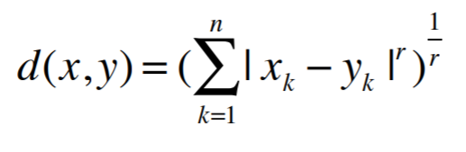
- r = 1: The formula is Manhattan Distance.
- r = 2: The formula is Euclidean Distance
- r = ∞: Supremum Distance
Pearson Correlation Coefficient
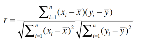
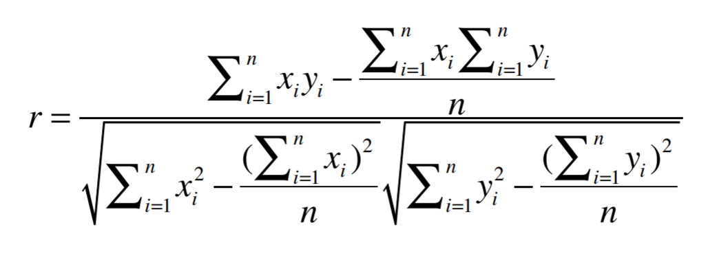
We see that users have very different behaviors when it comes to rating bands, they give different ranges of these bands(some are grade inflation, some not). One way to fix this problem is to use the Pearson Correlation Coefficient.
Cosine similarity
-
If the data is subject to grade-inflation (different users may be using different scales) use Pearson.
-
If your data is dense (almost all attributes have nonzero values) and the magnitude of the attribute values is important, use distance measures such as Euclidean or Manhattan.
-
If the data is sparse consider using Cosine Similarity.
Implementing k-nearest neighbors in Python
When we are relying on a single “most similar” person. Any quirk that person has is passed on as a recommendation. One way of evening out those quirks is to base our recommendations on more than one person who is similar to our user. For this we can use the k-nearest neighbor approach.
Chapter 3 Implicit Ratings and Item Based Filtering
Explicit ratings & Implicit ratings
Explicit ratings are when the user herself explicitly rates the item.
For implicit ratings, we don’t ask users to give any ratings—we just observe their behavior. An example of this is keeping track of what a user clicks on in the online New York Times. Another implicit rating is what the customer actually buys. Amazon also keeps track of this information and uses it for their recommendations “Frequently Bought Together” and “Customers Who Viewed This Item Also Bought”.
What can we use as implicit data when we are observing a person’s behavior at a computer?
Web pages: clicking on the link to a page, time spent looking at a page, repeated visits, referring a page to others, what a person watches on Hulu
Music players: what the person plays, skipping tunes, number of times a tune is played
Which is more accurate: explicit or implicit?
Problems with explicit ratings
Problem 1: People are lazy and don’t rate items
Problem 2: People may lie or give only partial information
Problem 3: People don’t update their ratings.
Problems with implicit ratings
Amazon’s purchase history can’t distinguish between purchases for myself and purchases I make as gifts.
Consider a couple sharing a Netflix account. He likes action flicks with lots of explosions and helicopters; she likes intellectual movies and romantic comedies. If we just look at rental history, we build an odd profile of someone liking two very different things.
So we can gain a substantial amount of information from a person’s purchase history.
User-based filtering
We are comparing a user with every other user to find the closest matches.
There are two main problems with this approach:
-
Scalability. As we have just discussed, the computation increases as the number of users increases. User-based methods work fine for thousands of users, but scalability gets to be a problem when we have a million users.
-
Sparsity. Most recommendation systems have many users and many products but the average user rates a small fraction of the total products. For example, Amazon carries millions of books but the average user rates just a handful of books. Because of this the algorithms we covered in chapter 2 may not find any nearest neighbors.
Item-based filtering
Suppose I have an algorithm that identifies products that are most similar to each other.
User-based vs Item-based
In user-based filtering we had a user, found the most similar person (or users) to that user and used the ratings of that similar person to make recommendations.
In item-based filtering, ahead of time we find the most similar items, and combine that with a user’s rating of items to generate a recommendation.
User-based filtering is also called memory based collaborative filtering. Why? Because we need to store all the ratings in order to make recommendations.
Item-based filtering is also called model-based collaborative filtering. Why? Because we don’t need to store all the ratings. We build a model representing how close every item is to every other item!
Adjusted Cosine Similarity
To compensate for this grade inflation we will subtract the user’s average rating from each rating. This gives us the adjusted cosine similarity formula below:
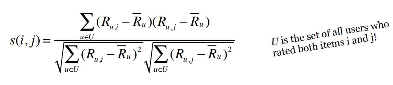
This formula is from a seminal article in collaborative filtering: Item-based collaborative filtering recommendation algorithms.
Now that we have this nice matrix of similarity values, it would be dreamy if we could use it to make predictions! We will use this formula to make prediction:
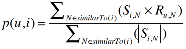
It’s just a weighted(weight is similarity) rating.
For this to work best, rating about one item should be a value in the range -1 to 1.
Slope One Algorithm
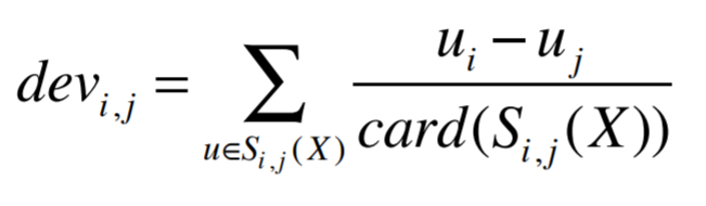
Another popular algorithm for item-based collaborative filtering is Slope One. A major advantage of Slope One is that it is simple and hence easy to implement. Slope One was introduced in the paper: Slope One Predictors for Online Rating-Based Collaborative Filtering. This is an awesome paper and well worth the read.
- Computing deviation between every pair of items
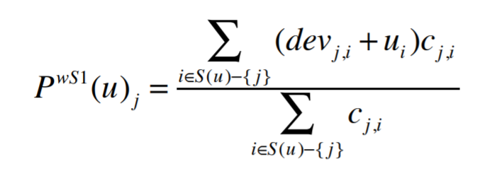
- Making predictions with Weighted Slope One
Chapter 4 Classification
In the previous chapters we used people’s ratings of products to make recommendations. In this chapter we use attributes of the products themselves to make recommendations. This approach is used by Pandora among others.
Data normalization
One common method of normalization involves having the values of each feature range from 0 to 1.
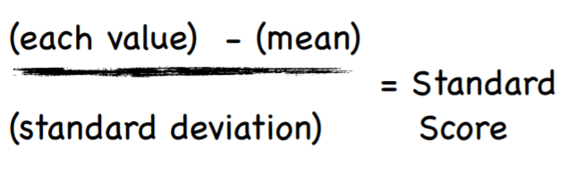
Or, We can standardize a value using the Standard Score (aka z-score) which tells us how many deviations the value is from the mean.
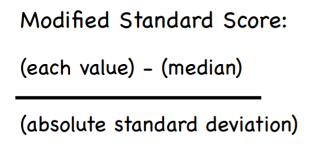
Sometimes the mean is greatly influenced by outliers. Because of this problem with the mean, the standard score formula is often modified.
odds and ends
In this chapter we talked the importance of normalizing data. This is critical when attributes have drastically different scales (for example, income and age). In order to get accurate distance measurements, we should rescale the attributes so they all have the same scale.
While most data miners use the term ‘normalization’ to refer to this rescaling, others make a distinction between ‘normaliza-tion’ and ‘standardization.’ For them, normalization means scaling values so they lie on a scale from 0 to 1. Standardization, on the other hand, refers to scaling an attribute so the average (mean or median) is 0, and other values are deviations from this average (standard deviation or absolute standard deviation). So for these data miners, Standard Score and Modified Standard Score are examples of standardization.