A guide to practical data mining, collective intelligence, and building recommendation systems by Ron Zacharski.
Chapter 5 Further Explorations in Classification
This chapter examines several other algorithms for classification including kNN and naïve Bayes. We look at the power of adding more data.
Leave-One-Out
In the machine learning literature, n-fold cross validation (where n is the number of samples in our data set) is called leave-one-out.
Benefit
- at every iteration we are using the largest possible amount of our data for training.
- deterministic.
10-fold cross validation is called non-deterministic because when we run the test again we are not guaranteed to get the same result. The reason we get different results is that there is a random component to placing the data into buckets.
Disadvantages
- the computational expense of the method
- stratification
Kappa Statistic
The Kappa Statistic will tell us how much better the real classifier is compared to this random one. The formula is
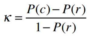
where P(c) is the accuracy of the real classifier and P(r) is the accuracy of the random one.
the kNN algorithm
One problem with the nearest neighbor algorithm occurs when we have outliers. One way to improve our current nearest neighbor approach is instead of looking at one nearest neighbor we look at a number of nearest neighbors—k nearest neighbors or kNN.
At the side of that Mexican road, I got to talking with Eric Brill about improving the performance of algorithms. His view is that you get more of an improvement by getting more data for the training set, than you would by improving the algorithm.
This isn’t to say that you shouldn’t pick the best algorithm for the job. As we have already seen picking a good algorithm makes a significant difference. However, if you are trying to solve a practical problem (rather than publish a research paper) it might not be worth your while to spend a lot of time researching and tweaking algorithms.
Chapter 6 Naïve Bayes and Probability Density Functions
This chapter introduces the Naïve Bayes Classifier.
P(h), the probability that some hypothesis h is true, is called the prior probability of h.
| P(h | d) is called the posterior probability of h. |
Chapter 7 Naïve Bayes and unstructured text
This chapter explores how we can use Naïve Bayes to classify unstructured text. Can we do sentiment analysis of movie reviews to determine if the reviews are positive or negative?
Classifying unstructured text
We have also looked at classification systems that use attributes like height, weight, how people voted on a particular bill. In all these cases the information in the datasets can easily be represented in a table.
This type of data is called “structured data”—data where instances (rows in the tables above) are described by a set of attributes (for example, a row in a table might describe a car by a set of attributes including miles per gallon, the number of cylinders and so on). Unstructured data includes things like email messages, twitter messages, blog posts, and newspaper articles. These types of things (at least at first glance) do not seem to be neatly represented in a table.
Chapter 8 Clustering
This chapter looks at two different methods of clustering: hierarchical clustering and kmeans clustering.
what is clustering
But what happens if I don’t know the possible labels?
This task is called clustering. The system divides a set of instances into clusters or groups based on some measure of similarity. There are two main types of clustering algorithms.
k-means clustering
For one type, we tell the algorithm how many clusters to make.
hierarchical clustering
For the other approach we don’t specify how many clusters to make.
Instead the algorithm starts with each instance in its own cluster. At each iteration of the algorithm it combines the two most similar clusters into one. It repeatedly does this until there is only one cluster.
The basic k-means algorithm is:
- select k random instances to be the initial centroids
- REPEAT
- assign each instance to the nearest centroid. (forming k clusters)
- update centroids by computing mean of each cluster
- UNTIL centroids don’t change (much).
We stop when the centroids don’t change. This is the same condition as saying no point are shifting from one cluster to another. This is what we mean when we say the algorithm ‘converges’.
Because of this behavior of the algorithm, we can dramatically reduce its execution time by relaxing our criteria of “no points are shifting from one cluster to another” to “fewer than 1% of the points are shifting from one cluster to another.” This is a common approach!
K-means is an instance of the Expectation Maximization (EM) Algorithm, which is an iterative method that alternates between two phases. We start with an initial estimate of some parameter. In the Kmeans case we start with an estimate of the centroids. In the expectation (E) phase, we use this estimate to place points into their expected cluster. In the Maximization (M) phase we use these expected values to adjust the estimate of the centroids. If you are interested in learning more about the EM algorithm the wikipedia page is a good place to start.
K-means is not guaranteed to reach the optimal solution, but only to find the local optimum.
To determine the quality of a set of clusters we can use the sum of the squared error (SSE). This is also called scatter. Here is how to compute it: for each point we will square the distance from that point to its centroid, then add all those squared distances together.